Probability theory

Classical probability

In a classical probabilistic space you have events and a probability measure:

But you want numerical data, so you study random variables: functions

such that

for every open set $A=\{z\in \mathbb C: a $$ sup_{\Omega} \{f(\omega)\}< \infty. $$

They constitute the algebra $L^{\infty}(\Omega, \Sigma,P)$, and the expected value for any random variable $g$, defined by

plays the role of a linear functional

In fact, it is not only an algebra, but a commutative von Neumann algebra, and $E_P$ is what it is called a faithful, normal state (see Quantum Probability Theory, from Hans Maasen, for details).

There is a theorem called the Gelfand-Naimark theorem which applied to a von Neumann algebra with a normal, faithful state let us recover the original probabilistic space. That is to say: all the data is inside the von Neumann algebra and the linear functional.

Sketch of the construction: if we begin with an algebra $\mathcal{A}$ (it could be $L^{\infty}(\Omega, \Sigma, P)$ or not) we recover a $\sigma$-algebra $\Sigma$ by selecting all the $p\in \mathcal{A}$ such that $p^2=p=p^*$. Think if $p \in L^{\infty}$ is like that, $p(\omega)=0$ or $p(\omega)=1$, and $p$ works like and indicator function of a set $A_p \in \Sigma$. The inclusion $\subseteq$ relation in $\Sigma$ is recovered by means of the relation: $p\subseteq q$ iff $p\cdot q=p$. And so we can recover the elementary events and the sample space $\Omega$.

Quantum probability

I have written two times about quantum probability. I have to re-read and merge both text (I don't know which is better)

Text 1:

Coming from above. And now, here comes the key idea: making a mental effort you can see any $f\in L^{\infty}$ like an operator on a Hilbert space. What Hilbert space? Well, is $L^2(\Omega,\Sigma,P)$, and as weird as it can look, you can think that is nothing else than $\mathbb C^n$ when $\Omega$ has cardinal $n$. So, in a finite $\Omega$ you can associate to $f$ the linear map

simply defined like the diagonal matrix whose entries are the values of $f$.

This way we distinguish a subset $\mathcal{F}$ of $End(\mathbb C^n)$ which is a subalgebra. And it turns out that if you take any other subalgebra being a von Neumann algebra and with a faithful, normal state, and if this algebra is non-commutative, what you recover with the Gelfand-Naimark theorem is a quantum version of probability. These non-commutative matrices are the observables (the random variables, if you want) of this theory.

Let's try with an example. Consider $\Omega=\{a,b,c\}$ (abstract results of an experiment), $\Sigma=2^{\Omega}$ and $P$ such that $P(a)=P(b)=1/4$ and $P(c)=1/2$. We can look at a random variable $f\in L^{\infty}(\Omega, \Sigma, P)$:

such that $f(a)=2$, $f(b)=3$ and $f(c)=1$. The meaning is something like putting a numerical tag over every $x\in \Omega$.

But we can think in a more active visualization of all this stuff. Imagine that $a,b,c$ are physical features of football players.

I can express a player with three numbers $\alpha_1, \alpha_2, \alpha_3$, and element of $\mathbb C^3$. Players, in general, are "superposition" of features: none of them is "only velocity". And also they are not normalized states: there can be a player who is bad at everything. The elements of the Hilbert space are like particular players and the elements of the corresponding projective space (pure states) are ideal classes of players (goalkeeper, striker, left back,...). It is as if we relativize the player with respect to himself (as when I used to say I was a climber cyclist, even if I was a worse climber than a professional sprinter).

What is the role of our function $f$? It would be like a treatment to change these features (a training system or a drug): you can amplify any of the features with different coefficients.

• The function $f$ applied to a player by means of $M_f$ returns a new player with improved (or worsened) features.

• A state $\omega$ (a class of players) acts as a functional on the algebra $\mathcal{F}$ and $\omega(f)$ is the average improvement of the treatment $f$ over the player of type $f$.

If several treatments changes features in a _isolated way_, like the previous one, you can apply them to the player in the order you want.That is, they commute. But we can admit other treatments which act in a more complicated way, i. e., no diagonal matrices than may not commute. Our $f$ is a map $f:\mathbb C^n \longmapsto \mathbb C^n$ sending a player configuration to the new one after the treatment. It would correspond to a matrix

That is, we are identifying $f$ with an element $M_f \in End(\mathbb C^n)$. That is, we have a map

such that $\mathcal{M}(f)=M_f$.

But, in fact, $a,b,c$ can also be identified with elements of $End(\mathbb C^n)$:

And the evaluation process

corresponds to

This operation has a name, is the Frobenius inner product, related to the trace:

Even $P$ is an element of $End(\mathbb C^n)$,

being $Tr(M_f M_P)$ the expected value of $f$. In fact, you can see _evaluation of $f$ in $a$_ like the expected value of $f$ over a degenerate probability measure concentrated at $a$:

Moreover, the probability of an event, for example $\{a\}$, is the expected value of a degenerate random variable concentrated at $a$

Matrices such that $B^2=B$. They are typically the ones associated with elements of $\Omega$ or $\Sigma$, when we consider $B\in \mathcal{M}(L^{\infty})$. But if we expand our _algebra of interest_ from $\mathcal{M}(L^{\infty})$ to something bigger we obtain objects that do not belong to the original sample space or $\sigma$-algebra, but behave like if they do.

For example, consider the matrix

We can try to evaluate our $f$ in $B$, be mean of

and we obtain 2'5. Something between $f(a)$ and $f(3)$. It looks like if we are filling the holes of the sample space $\Omega$.

Another key idea to develop: as subspaces and even as linear maps, events and states are the same. I compute the probability of an event given a state by projecting the state vector over the event subspace: the squared length is the probability and the resulting vector is the new state, or by means of the trace if I consider them operators. They should be treated on the same footing.

Text 2:

With classical probability

We are going to analyse, from the beginning, the Stern-Gerlach experiment from a mathematical viewpoint, and try to see why is natural the formulation of QM. Imagine that electrons have an internal configuration that can be observed with a Stern-Gerlach device ($SG$) when they are shot with an electron gun. We align the machine with the $z$ axis (we call this configuration $SG_z$) and it gives us two outputs when electrons arrive: for example, red and green. Our first idea would be to think that there are two kinds of electrons or two states of the electron.

From the point of view of set theory, improved with basic probability theory, our first thought is: "ok, I have a set of electrons $\tilde{\Omega}$ and a map that sends their elements to the set $\{r,g\}$ with different frequencies. So, since there are (approximately) an infinite number of electrons, I can take a partition of $\tilde{\Omega}$ and shrink all data to a new set $\Omega=\{r,g\}$ with a probability measure $P$, and we would have no loss of information.

Then, we observe that if we have a copy of this machine and rotate it (or keep it fixed and rotate the gun that shoot the electrons in the opposite direction) to the $x$ axis (let's call $SG_x$ to this second machine) then we obtain two other outputs (big and small, for example) with a new probability distribution $P'$. If we assume a classical behavior of the states of the electron, i.e., we can use machine $SG_z$ on an electron and then machine $SG_x$ on the same electron and that does not change the state itself, we can obtain a joint probability distribution $\tilde{P}$, and conclude that there are four different states:

with a new probability function. Our new set appears like a Cartesian product of the previous "sets of possibilities".

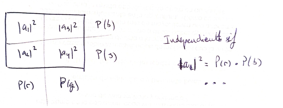
Observe that the joint distribution is not necessarily

being this the case only when the variables are independent. For example, maybe there is a correlation between being red and being big.

A different approach

All of this could have been translated into math in a very different way, far more complicated, but that it will pay off later.

A finite set $B$ with $N$ elements can be viewed as a Hilbert space

with inner product

This way we have "enriched" the set:

1. we conserve the original elements of the set, codified in the rays through the canonical basis; but we get new objects, the superposition of the elements. This new objects may not have an interpretation for us, at a first glance.

2. And we also have a measure of "how independent" this objects are: the inner product. For example, the original elements are totally independent, since their inner product is 0.

Let's come back to Stern-Gerlach. Instead of thinking as before in the set $\Omega=\{r,g\}$, we take the Hilbert space

with the usual inner product.

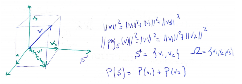
The canonical basis elements of $\mathcal{H}_1$ (or better said, the rays through them) will represent the states $r$ and $g$, and the probability function $P$ will be encoded in a unitary vector $s_1 \in \mathcal{H}_1$ (or better said, the ray through it) in such a way that

represents the probability of obtaining the output $r$ when using the first machine. And the same for $g$. Observe that we are treating on an equal footing the states ($r$ or $g$) and the probability measure.

So far, two questions can arise:

• We have chosen in $\mathcal{H}_1$ the usual inner product (equivalent to $\|\cdot \|_2$). Why not other inner product or even why not a simpler mathematical object like an absolute value norm? That is, why don't we take, for example, $\|v\|_1=|v_1|+|v_2|$ and encode probabilities in $\|proj_r(s_1)\|_1$ without the square? Well, the only $p$-norm satisfying the parallelogram rule is $\|\cdot\|_2$, and this rule is needed to form an inner product from the norm. The finer approach of inner product will be needed later because it let us use further mathematics concepts (orthogonality, unitary Lie groups,...). Moreover, even intuitively the inner product approach is desirable because it gives us a measure of the independence of the elements represented by the rays in the Hilbert space.

• Why don't we use real numbers and take as probabilities the absolute values of the component instead of the square? Once we fix the use of the 2-norm, we need to deal with amplitudes (i.e., numbers whose square give probabilities) because we want to keep with us the addition of probabilities for incompatible events, from the classical setup.

• And also, why complex numbers in QM?

Within this approach to sets as Hilbert spaces, subsets are encoded as subspaces, the union of sets is translated as the direct sum of subspaces, intersection of sets as intersections of subspaces and the complement of a set as the orthogonal complement of the subspace.

Random variables vs operators

Let's continue with $(\mathcal{H}_1, \langle | \rangle{}{})$. If we had numerical data instead of qualitative one (i.e., suppose that instead of "red" and "green", our machine give us two fixed values 0'7 and 1'8, or in other words, a random variable) we would codify this, within this new approach, in the idea of an operator. That is, a linear map

such that

i.e.,

The random variable registers the idea of a measurement. This new approach to them may look very artificial, but it retains the same information that the classical probability approach:

• We recuperate the values, for example for $r$, with

• The expected value of $F$, provided that probabilities are given by the vector $s_1$, would be

When we take our second machine $SG_x$ we have other Hilbert space, say $\mathcal{H}_2$, and other state $s_2 \in \mathcal{H}_2$ encoding probabilities of $b$ and $s$. Suppose that this machine also gives numerical values, so that we have another operator $G:\mathcal{H}_2\mapsto \mathcal{H}_2$, also diagonal in the canonical basis of $\mathcal{H}_2$.

If we assume, as before, a classical behavior of the states, we can model this with a new Hilbert space

whose basis will be denoted by $\{rb, rs, gb, gs\}$. This tensor product plays the role of cartesian product in the previous set up.

We can think that the state describing the system would be

but in fact this is only an special case when the two machines are yielding the equivalent to "independent variables" (the joint probability is the product of the probabilities). In general, it is valid any $\Psi \in \mathcal{H}_1 \otimes \mathcal{H}_2$ provided that the coefficients in the linear combination

are such that

where the second and the fourth equations could be deduced, so we can remove it.

The random variable represented by the operator $F$ corresponds here to $F\otimes Id$ (Kronecker product), and $G$ to $Id \otimes G$.

________________________________________

________________________________________

________________________________________

Author of the notes: Antonio J. Pan-Collantes

antonio.pan@uca.es